Software
Table of contents
Vision
Hardware
Our video system is mainly composed of 6 camera tripod stands with a:
- ZED 2 (Stereo Camera)
- Jetson Nano (Compute Module)
- Wifi Antenna (Wireless Data Transmission)
- Battery Pack (Power Supply)
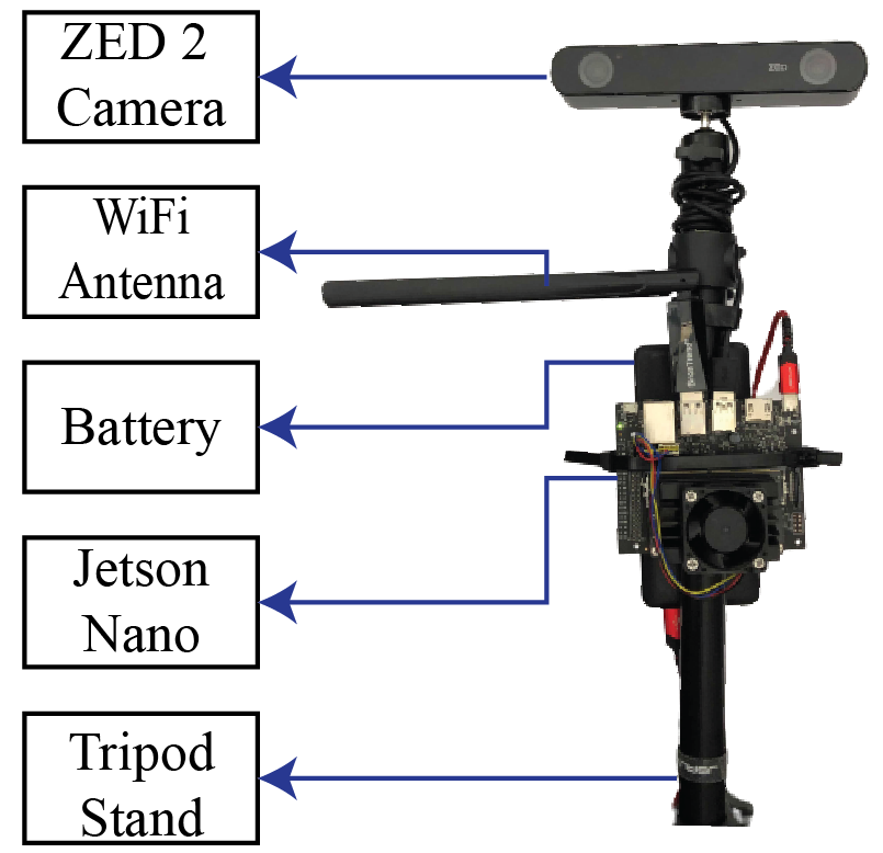
positioned around the tennis court to capture ball movements.
All jetsons should have:
- Ubuntu 18.04
- ROS Melodic
- ZED SDK
- OpenCV 4.5.2+ (with CUDA)
- Catkin workspace with
jetson_masterbranch - Username: jetson-nano-<ID>
- Password: 1111
- IP:
192.168.1.10<ID>(IDs range from 1 to 6)
Static IP
We also have a 5GHz wifi router (core-robotics-net-5G) that allows the stands to be connected to a shared network and transmit data to the wheelchair computer. All jetsons should have a static IP based on their assigned ID like 192.168.1.10<ID>, so jetson with ID 3 should have IP 192.168.1.103 and should be accessible through SSH at jetson-nano-3@192.168.1.103. Note that we are actually assigning the IP address to the long-range wifi antennas and not the jetson internal wifi module. We assign the antenna’s MAC address to a static IP within the router’s admin settings. Please ask the project lead if you need the router password. Each antenna and jetson should have a tag with an ID that it maps to, so don’t interchange antennas and jetsons.
The master computer should always have the antenna with tag 0 in order to map it to 192.168.1.100. This is important for roscore and time sync.
The jetson should automatically connect to core-robotics-net-2 on boot if the network avialable. You can find all the jetson connected by using nmap -sP 192.168.1.* | grep "192.168.1.10". If a jetson is not connected, you need to ssh into the jetson (likely through ethernet cable) and use sudo nmcli d wifi connect core-robotics-net-2_5G password ogmcglab.
Time Sync
In order for all the Jetsons to have sync’d time for pose estimates, we use chrony and let the master computer be the main NTP server.
Setup New Jetson
On a 32Gb SD Card, flash the image with all the software requirements from this link. Now to update the username for the jetsons, we can follow the steps given in this thread and change the home directory with a renamed copy of the original folder. The password should be changed by logging into the root of the system.
To set up the ROS Networking on the Jetsons, change ~/.bashrc and add: export ROS_MASTER_URI=http://192.168.1.100:11311 and export ROS_HOSTNAME=<Jetson IP>. Make sure Jetson is loaded with all the required packages.
Calibration
To get the camera’s relative position within the world, we use Apriltag calibration to get accurate pose estimates. We created a box covered in unique Apriltag bundles so that we can calibrate the cameras with a pre-measured box in a known position in the world. All this functionality is located in the ball_calibration package.
Refer to court calibration section for main details.
Ball Detection
Our current method of detecting an orange tennis ball is to find the center of the “largest moving orange object” within an image. A simple explanation of the approach involves:
- For left and right images of the stereo camera:
- Perform background subtraction (find moving objects)
- Perform HSV color thresholding (find orange objects)
- Determine the largest area that is moving and contains orange (find largest)
- Find the center of this area
- Perform stereo depth estimation based on left and right centers position
- Convert to pose estimate with predicted measurement covariance
This pose estimate then is sent to the Extended Kalman Filter (EKF) for processing.
We perform this detection process on the jetsons since transmitting image data is quite expensive. Since the jetsons aren’t very powerful, we had to optimize our detections code by using GPU and incorporating some other complex optimizations.
Position Tracking
Currently, for fusing all the camera’s position estimates we use a modified version of robot_localization’s EKF that accounts for the ball’s ballistic dynamics called ball_localization. We also incorporated the ability to rollout the ball trajectory into the future by iteratively calling the EKF’s predicting method. Setting for the EKF can be tuned within this yaml based for of robot_localization.
We tune the EKF, especially the ball bounce parameters, using a script that evualates the bag position history versus the EKF rollout for a particular time using this testing script
Wheelchair Navigation Stack
The motion of ESTHER’s wheelchair base can be modeled as a differential drive base that is equipped with three different sensors to determine the robot’s state in the world.
- Motor encoders provide the velocity and position of each wheel @ 250 Hz
- Inertial Measurement Units (IMU) provide used to obtain the linear velocity, angular velocity, and orientation of the motion base @ 400 Hz
- LiDAR sensors provide an egocentric 360° point cloud with a 30° vertical field of view @ 20 Hz
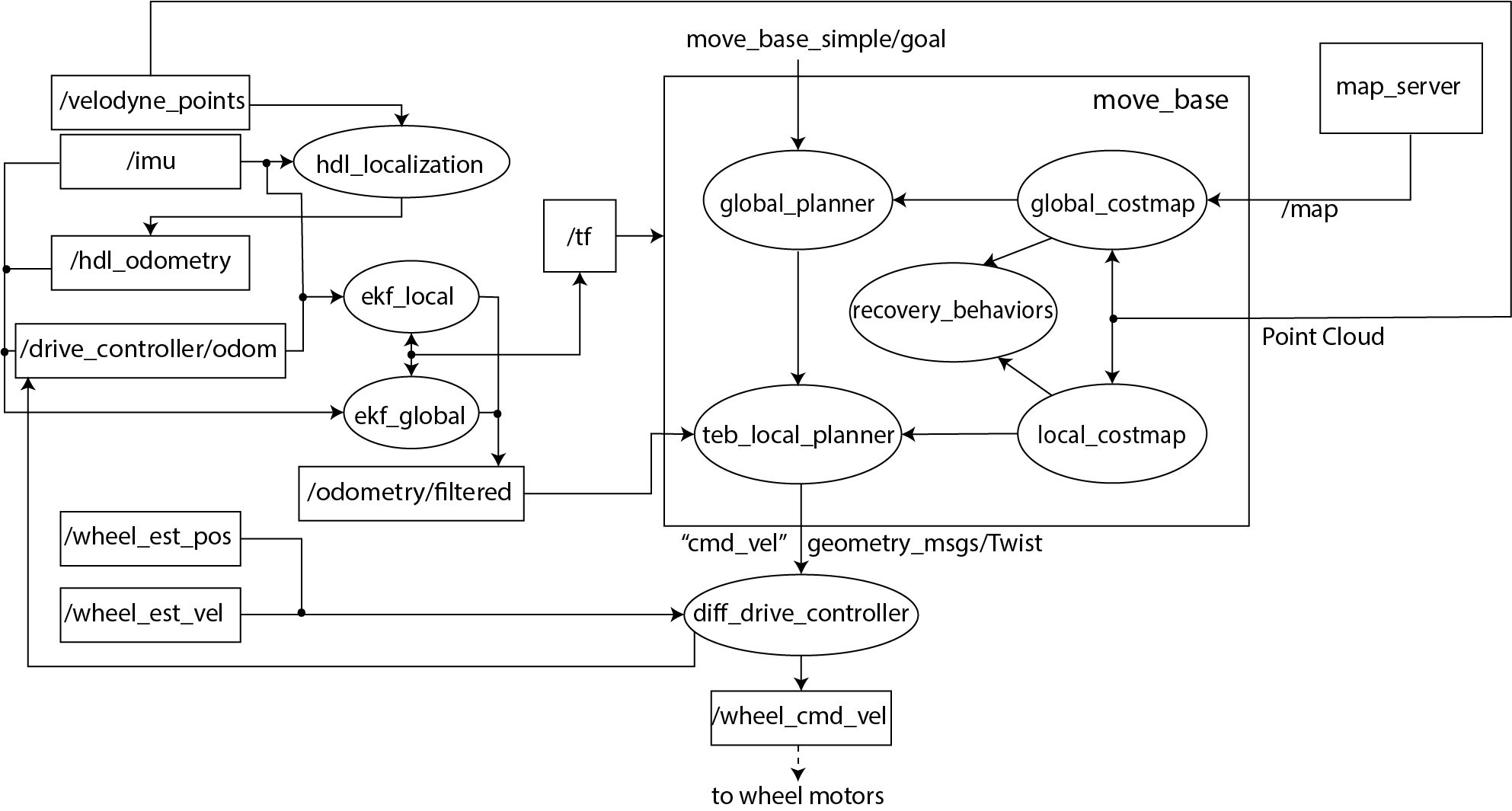
We customized ROS’s Navigation Stack to fit our requirements. Our system produces local and global state estimates of the robot’s pose in the world from sensor data using two EKF state estimation nodes. The complete navigation stack can be visualized in image below.
Localization
For localizing the wheelchair, we first create a map of the environment offline by recording IMU and 3D point cloud data while manually driving the wheelchair around at slow speeds. The hdl_graph_slam package is used to create the Point Cloud Data (PCD) map from the recorded data for online use. Afterward, we use a point cloud scan matching algorithm from the hdl_graph_slam package to obtain an odometry estimate based on the LiDAR and IMU readings. A differential drive controller gives a second odometry estimate from the wheel encoder data and IMU readings.
Following guidance from the robot_localization package, we fuse these estimates to get the current state of the wheelchair. ekf_local from the figure above fuses only the continuous data (i.e. IMU data and odometry estimate from the differential drive controller). This EKF provides a continuous odometry estimate, which can be used execute path plans on the robot’s mobile base. ekf_global from the figure above fuses data from all three sources (i.e. the odometry estimate from hdl_localization, the odometry estimate from differential drive controller, and the IMU data). The purpose of ekf_global is to eliminate the drift that might accumulate overtime in the robot’s position.
As per ROS’s conventions, ekf_local provides a continuous, smooth transform without any jumps or discontinuities between the “odom” frame and the mobile base frame. ekf_global eliminates the accumulated drift in the robot position by providing a transform between the “odom” frame and the “world” frame. This can cause jumps and discontinuities in the output of the estimate, however it is not a concern as we are not executing motions in this frame of reference.
Planner
The move_base package from the ROS Navigation Stack is used to move the mobile base around the environment. Inside move_base, we use the default global planner global_planner which uses Dijkstra’s algorithm to make a global plan, and the Timed Elastic Band (TEB) planner teb_local_planner to make a local plan. The differential drive controller converts the commanded twist from the teb_local_planner to wheel velocities. A low-level PID velocity controller tracks the commanded wheel velocities.
Arm
Calibration
The Barrett WAM traditionally uses relative encoders. Therefore, for accurate control, the arm needs to be calibrated properly. This guide from Barrett WAM can be used to do zero-calibration of the arm. Additionally, it will also be useful if gravity calibration is also performed. However, with the tennis racket mounted on the robot, gravity calibration is difficult as the racket will obstruct the calibration procedure.
Before running any code on the arm, care should be taken to ensure that the arm is at home position. The arm is at home position when joints J1, J3, J4, J5, J6 and J7 are at 0 rad, joint J2 is at -2 rad, joint J4 is at π rad. For visualizing follow this link.
Controller
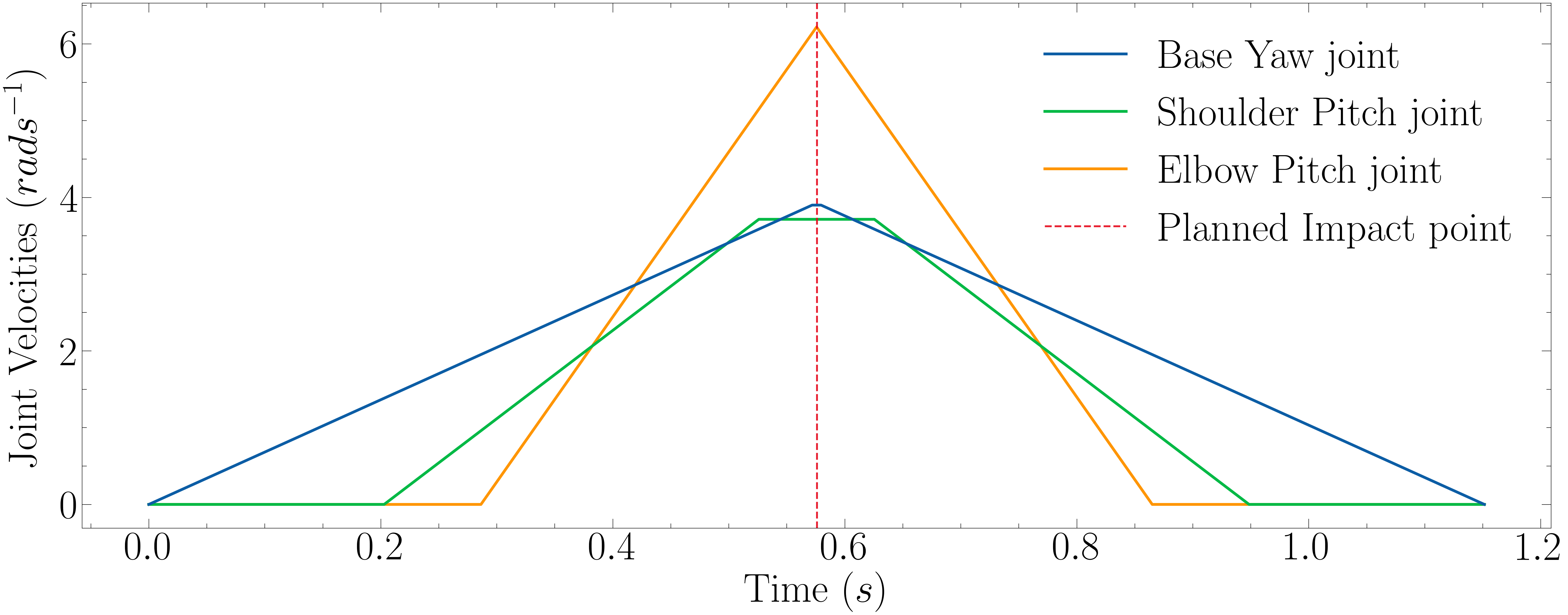
To maximize the joint velocities when the robot makes contact with the ball, we use a trapezoidal trajectory profiler. The trapezoidal trajectory profiler takes in a start point, mid point, and end point. Each joint starts moving with maximum acceleration until it reaches either maximum velocity or the velocity from which it can decelerate in time to stop at the end position. Each joint trajectory is shifted in time to make sure that every joint is moving at its maximum velocity when the racket makes contact with the ball at the midpoint of the swing. Joints’ position, velocity, and acceleration limits are accounted for while creating the trapezoidal profiles. The joints’ trajectories are sent from the onboard computer to the WAM computer which uses a PID controller to execute the trajectory on the arm. An example velocity profile is shown in the figure below.
Strategizer
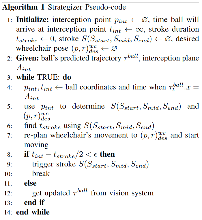
The strategizer works as follows:
- The strategizer first determines the interception point by finding the point at which the ball will cross the plane that goes through the center of the robot.
- Based on the interception point, the strategizer determines the stroke parameters which is parameterized by three points:
- Start point: joint space configuration at the swing’s beginning
- Contact point: joint space configuration at ball contact
- End point: joint space configuration at the swing’s completion These points are determined such that the arm is fully extended at contact point to maximize racket-head linear velocity while each joint is traveling at the maximum possible speed and staying within each individual joint’s position, velocity, and acceleration limits.
- As the arm would be fully extended at the contact point, the corresponding wheelchair position is geometrically determined using the robot kinematics and the interception point. Once, the position is determined the wheelchair is commanded to go to that position.
- Lastly, the strategizer identifies the exact time to trigger the stroke using the stroke duration and the time the ball takes to reach the interception point. The text in the paper is updated to make the process more clear.
The pseudocode for the strategizer is provided below.
Now check out the gallery page to see how to see some videos of how well the system works.